How to take a quick look at a dataset

This post helps you make some basic exploration on a dataset. Specifically, it helps you do the following using Python.

1. Print the first few rows and see how data is organised under different columns

2. Take a slightly technical view of the dataset. Check how many rows and columns are there, what are the different data types etc

3. Get a statistical summary of the numerical attributes in the data set

4. Plot histograms of the numerical attributes. Histograms provide insights that may not be evident from the statistical summary of the data.

Load the dataset

In this article, let's use the popular housing dataset to explore the points mentioned above. The dataset has information on house prices in different housing districts in California, USA. The dataset is available on Github. If you are using Google Colab for running your code, you can directly load the data from Github. There is no need to save a local copy on your hard disk.

To load the dataset, type the following in your Colab document.

import pandas as pd

url = 'https://raw.githubusercontent.com/puttym/machine-learning/master/housing.csv'
housing = pd.read_csv(url)

The read_csv() method reads a CSV file to a Pandas dataframe, and returns a dataframe object. In our code, the returned dataframe object is assigned to the variable housing.

We are now in a position to look at the data.

1. Print the first few rows of the dataset

We can print the first five rows of the dataset by using the head() method.

housing.head()

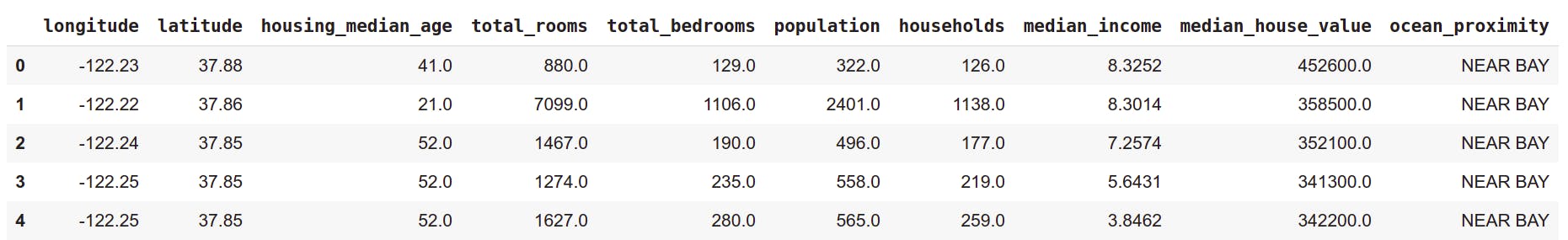
In the dataset, each row provides information on one housing district. For each housing district, we have general information like the number of households and population. The dataset also mentions how many rooms are there in the entire district, and how many of them are bed rooms. We can also find economic indicators like median income and median house value.

There are two types of information regarding the location of the housing district. One of them attaches a lat-long pair to each district, while the other tells us how close the district is to the ocean. We might guess that districts closer to the ocean have higher median house values.

2. Get slightly technical

Let's now look at some of the technical aspects of the dataset. We do this by invoking the info() method.

housing.info()

Output:

class 'pandas.core.frame.DataFrame'>
RangeIndex: 20640 entries, 0 to 20639
Data columns (total 10 columns):
 #   Column              Non-Null Count  Dtype  
---  ------              --------------  -----  
 0   longitude           20640 non-null  float64
 1   latitude            20640 non-null  float64
 2   housing_median_age  20640 non-null  float64
 3   total_rooms         20640 non-null  float64
 4   total_bedrooms      20433 non-null  float64
 5   population          20640 non-null  float64
 6   households          20640 non-null  float64
 7   median_income       20640 non-null  float64
 8   median_house_value  20640 non-null  float64
 9   ocean_proximity     20640 non-null  object 
dtypes: float64(9), object(1)
memory usage: 1.6+ MB

info() method prints a concise summary of the dataset. Specifically, it prints:

1. Number of rows and columns in the dataset
2. Column names (also called attributes)
3. Number of non-null entries under each column
4. Data type of values under each column

From the output of the info() method, we can make the following observations.

In the dataset, information is organised under 10 attributes and there are 20640 entries. All attributes, except total_bedrooms, have 20640 non-null entries, while total_bedrooms has only 20433 non-null entries. This means that the information on total_bedrooms is missing for 207 housing districts. Also, all attributes (except ocean_proximity) are of type float64 - a numeric datatype defined in Numpy.

ocean_proximity is of type object meaning that it can hold any kind of Python object (it just means that ocean_proximity can be just anything). However, since we loaded data from a CSV file, we can be certain that it's a text attribute. Also, we can guess that this is a categorical attribute and many instances have the same value. For example, all the five rows in the table above have the value NEAR BAY.

We can find all values of ocean_proximity by using the value_counts() method. The output shows that the attribute has five different values.

housing["ocean_proximity"].value_counts()

Output:

<1H OCEAN     9136
INLAND        6551
NEAR OCEAN    2658
NEAR BAY      2290
ISLAND           5
Name: ocean_proximity, dtype: int64

3. Get a statistical summary of the dataset

The describe() method provides a statistical summary of the numerical attributes.

housing.describe()

Output:

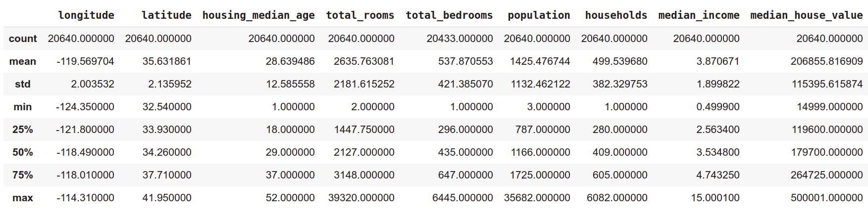
Rows like count, min, max, and mean are self explanatory. std is the standard deviation - a measure of dispersion of the values from the mean.

Rows 25%, 50%, and 75% represent the corresponding percentiles. To understand them, consider the households attribute in the table above. It says that 25% of the housing districts have less than 280 households, 50% of the districts have less than 409, and 75% of the districts have less than 605 . Similarly, 25% of the districts have population less than 787, 50% have population less than 1166, and 75% have population less than 1725.

The statistical summary also says something very interesting about a couple of attributes. The median income ranges between 0.5 and 15 indicating that these values are not in USD. Clearly, the actual values of income are transformed to fit within a scale of 0 -- 15, with 15 as the upper limit. That means, any income beyond a certain value is taken to be 15. Similalry, the the attribute housing_median_age is capped at 52.

The statistical summary also shows that the median house value is capped at USD 500,000. This is a limit imposed artificially within the dataset, and we can't expect to have such caps in actual market values of the houses. This fact should be taken seriously because our task is to predict the median house value for new districts that will be added. Because of this artificial upper limit, our machine learning algorithm might learn that the house values will not cross USD 500,000 and can potentially underestimate house values in certain districts.

4. Plot the histogram

While the describe() method gives a broad summary of the data, it's not of much use in answering questions like, How many housing districts have median house values in the range USD 90,000 - USD 100,000? One of the ways to answer such questions is to plot a histogram of the median house values and see how it is distributed. Instead of plotting one histogram, we can plot histograms of all the numerical attributes. Surprisingly, it is much easier to plot all histograms.

%matplotlib inline
import matplotlib.pyplot as plt
housing.hist(bins=50, figsize=(20, 15))
#plt.savefig("housing_histogram.png")
plt.show()

Output:

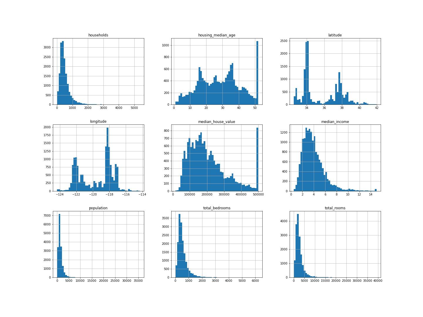
In all the histograms, the Y-axis represents the number of housing districts, and the X-axis in each histogram represents a unique numerical attribute. As you can see in the figure above, there are separate histograms for each numerical attribute like the median income, median house value etc. By looking at the histogram of median house value, we can say that a little more than 800 housing districts have median house value within the range USD 90,000 - USD 100,000. Similarly, around 700 districts have median house value within the range USD 190,000 and USD 200,000.

The histograms reiterate our earlier observations that the median house value is capped at USD 500,000, the median income is not in USD and is capped at 14, and housing median age is capped at 52.

Conclusion

In this article, we learnt four different ways of taking a quick look at a dataset. Each of them will give a different perspective: one just shows the data, the other provides a summary (how many rows, how many columns, what are the datatypes etc), the other gives a broad statistical summary of the numerical attributes, and the histogram graphically captures the distribution of data.

If you get any new dataset, you know what to do now!

Cover image: flickr.com/photos/volvob12b/42841524162

This article was originally posted on Sea of Tranquility.