


This article was originally posted by Shibsankar Das on the Neptune blog where you can find more in-depth articles for machine learning practitioners.
Generative Adversarial Networks (GANs) were first introduced in 2014 by Ian Goodfellow et. al. and since then this topic itself opened up a new area of research.
Within a few years, the research community came up with plenty of papers on this topic some of which have very interesting names :). You have CycleGAN, followed by BiCycleGAN, followed by ReCycleGAN and so on.
With the invention of GANs, Generative Models had started showing promising results in generating realistic images. GANs has shown tremendous success in Computer Vision. In recent times, it started showing promising results in Audio, Text as well.
Some of the most popular GAN formulations are:
- Transforming an image from one domain to another(CycleGAN),
- Generating an image from a textual description (text-to-image),
- Generating very high-resolution images (ProgressiveGAN) and many more.
In this article, we will talk about some of the most popular GAN architectures, particularly 6 architectures that you should know to have a diverse coverage on Generative Adversarial Networks (GANs).
Namely:
- CycleGAN
- StyleGAN
- pixelRNN
- text-2-image
- DiscoGAN
- lsGAN
GAN 101 and Vanilla GAN
There are 2 kinds of models in the context of Supervised Learning, Generative and Discriminative Models. Discriminative Models are primarily used to solve the Classification task where the model usually learns a decision boundary to predict which class a data point belongs to. On the other side, Generative Models are primarily used to generate synthetic data points that follow the same probability distribution as training data distribution. Our topic od discussion, Generative Adversarial Networks(GANs) is an example of the Generative Model.
The primary objective of the Generative Model is to learn the unknown probability distribution of the population from which the training observations are sampled from. Once the model is successfully trained, you can sample new, “generated” observations that follow the training distribution.
Let’s discuss the core concepts of GAN formulation.
GAN comprises of two independent networks, a Generator, and a Discriminator.
The Generator generates synthetic samples given a random noise [sampled from a latent space] and the Discriminator is a binary classifier that discriminates between whether the input sample is real [output a scalar value 1] or fake [output a scalar value 0].
Samples generated by the Generator is termed as a fake sample. As you see in Fig1 and Fig2 that when a data point from the training dataset is given as input to the Discriminator, it calls it out as a Real sample whereas it calls out the other data point as fake when it’s generated by the Generator.

Fig1: Generator and Discriminator as GAN building blocks
The beauty of this formulation is the adversarial nature between the Generator and the Discriminator.
The Discriminator wants to do its job in the best possible way. When a fake sample [which are generated by the Generator] is given to the Discriminator, it wants to call it out as fake but the Generator wants to generate samples in a way so that the Discriminator makes a mistake in calling it out as a real one. In some sense, the Generator is trying to fool the Discriminator.

Fig2: Generator and Discriminator as GAN building blocks
Let us have a quick look at the objective function and how does the optimization is done. It’s a min-max optimization formulation where the Generator wants to minimize the objective function whereas the Discriminator wants to maximize the same objective function.
Fig3 depicts the objective function being optimized. The Discriminator function is termed as D and the Generator function is termed as G. Pz is the probability distribution of the latent space which is usually a random Gaussian distribution. Pdata is the probability distribution of the training dataset. When x is sampled from Pdata , the Discriminator wants to classify it as a real sample. G(z) is a generated sample when G(z) is given as input to the Discriminator, it wants to classify it as a fake one.

Fig3: Objective function in GAN formulation
The Discriminator wants to drive the likelihood of D(G(z)) to 0. Hence it wants to maximize (1-D(G(z))) whereas the Generator wants to force the likelihood of D(G(z)) to 1 so that Discriminator makes a mistake in calling out a generated sample as real. Hence Generator wants to minimize (1-D(G(z)).

Fig4: Objective function in GAN formulation
CycleGAN:
CycleGAN is a very popular GAN architecture primarily being used to learn transformation between images of different styles.
As an example, this kind of formulation can learn:
- a map between artistic and realistic images,
- a transformation between images of horse and zebra,
- a transformation between winter image and summer image
- and so on
FaceApp is one of the most popular examples of CycleGAN where human faces are transformed into different age groups.
As an example, let’s say X is a set of images of horse and Y is a set of images of zebra.
The goal is to learn a mapping function G: X-> Y such that images generated by G(X) are indistinguishable from the image of Y. This objective is achieved using an Adversarial loss. This formulation not only learns G, but it also learns an inverse mapping function F: Y->X and use cycle-consistency loss to enforce F(G(X)) = X and vice versa.
While training, 2 kinds of training observations are given as input.
- One set of observations have paired images {Xi, Yi} for i where each Xi has it’s Yi counterpart.
- The other set of observations has a set of images from X and another set of images from Y without any match between Xi and Yi.

Fig5: The training procedure for CycleGAN.
As I have mentioned earlier there are 2 kinds of functions being learned, one of them is G which transforms X to Y and the other one is F which transforms Y to X and it comprises two individual GAN models. So, you will find 2 Discriminator function Dx, Dy.
As part of Adversarial formulation, there is one Discriminator Dx that classifies whether the transformed Y is indistinguishable from Y. Similarly, there is one more Discriminator Dy that classifies whether is indistinguishable from X.
Along with Adversarial Loss, CycleGAN uses cycle-consistency loss to enable training without paired images and this additional loss help the model to minimize reconstruction loss F(G(x)) ≈ X and G(F(Y)) ≈ Y
So, All-in-all CycleGAN formulation comprises of 3 individual loss as follows:

and as part of optimization, the following loss function is optimized.

Let’s take a look at some of the results from CycleGAN. As you see, the model has learned a transformation to convert an image of a zebra to a horse, a summer time image to the winter counterpart and vice-versa.

Following is a code snippet on the different loss functions. Please refer to the following reference for complete code flow.
CycleGAN
# Generator G translates X -> Y
# Generator F translates Y -> X.
fake_y = generator_g(real_x, training=True)
cycled_x = generator_f(fake_y, training=True)

fake_x = generator_f(real_y, training=True)
cycled_y = generator_g(fake_x, training=True)

# same_x and same_y are used for identity loss.
same_x = generator_f(real_x, training=True)
same_y = generator_g(real_y, training=True)

disc_real_x = discriminator_x(real_x, training=True)
disc_real_y = discriminator_y(real_y, training=True)

disc_fake_x = discriminator_x(fake_x, training=True)
disc_fake_y = discriminator_y(fake_y, training=True)

# calculate the loss
gen_g_loss = generator_loss(disc_fake_y)
gen_f_loss = generator_loss(disc_fake_x)

total_cycle_loss = calc_cycle_loss(real_x, cycled_x) + \
                   calc_cycle_loss(real_y,cycled_y)

# Total generator loss = adversarial loss + cycle loss
total_gen_g_loss = gen_g_loss + total_cycle_loss + identity_loss(real_y, same_y)
total_gen_f_loss = gen_f_loss + total_cycle_loss + identity_loss(real_x, same_x)

disc_x_loss = discriminator_loss(disc_real_x, disc_fake_x)
disc_y_loss = discriminator_loss(disc_real_y, disc_fake_y)
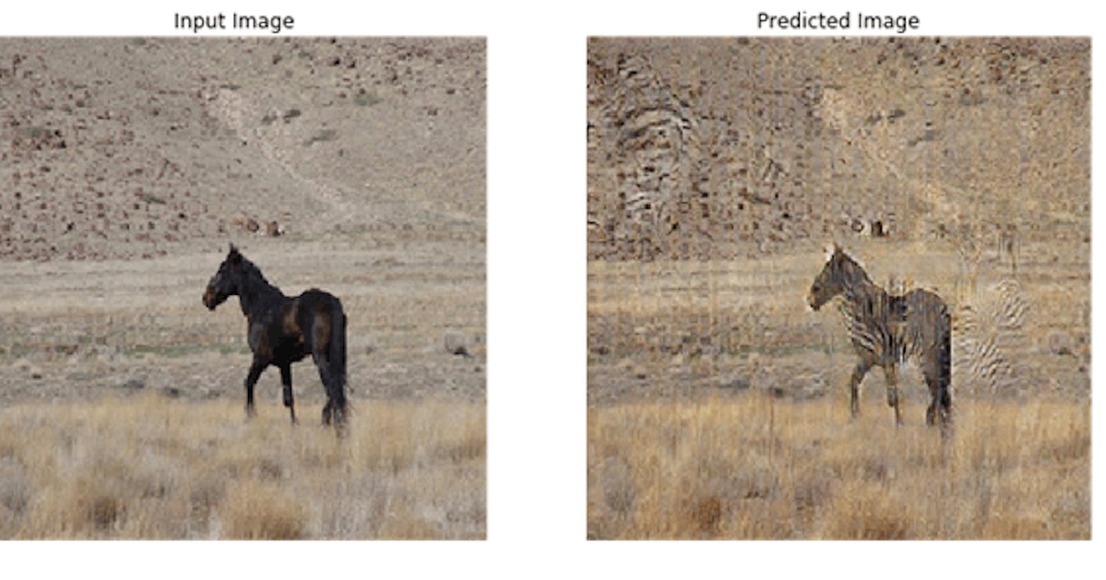
Following is an example where an image of horse has been transformed into an image that looks like a zebra.

References: Research Paper:
Tensorflow has a well-documented tutorial on CycleGAN. Please refer to the following URL as reference
tensorflow.org/tutorials/generative/cyclegan
StyleGAN:
Can you guess which image (from the following 2 images) is real and which one is generated by GAN?

The fact is that both the images are imagined by a GAN formulation called StyleGAN.
StyleGAN is a GAN formulation which is capable of generating very high-resolution images even of 10241024 resolution. **The idea is to build a stack of layers where initial layers are capable of generating low-resolution images (starting from 22) and further layers gradually increase the resolution.**
The easiest way for GAN to generate high-resolution images is to remember images from the training dataset and while generating new images it can add random noise to an existing image. In reality, StyleGAN doesn’t do that rather it learn features regarding human face and generates a new image of the human face that doesn’t exist in reality. If this sounds interesting, visit thispersondoesnotexist.com Each visit to this URL will generate a new image of a human face who doesn’t exist in the universe.

This figure depicts the typical architecture of StyleGAN. The latent space vector z is passed through a mapping transformation comprises of 8 fully connected layers whereas the synthesis network comprises of 18 layers, where each layer produces image from 4 x 4 to 1024 x 1024. The output layer output RGB image through a separate convolution layer. This architecture has 26.2 million parameters and because of this very high number of trainable parameters, this model requires a huge number of training images to build a successful model.
Each layer is normalized using Adaptive instance normalization (AdaIN) function as follows:

where each feature map xi is normalized separately, and then scaled and biased using the corresponding scalar components from style y. Thus the dimensionality of y is twice the number of feature maps on that layer.
References:
Paper: arxiv.org/pdf/1812.04948.pdf
Github: github.com/NVlabs/stylegan
PixelRNN
PixelRNN is an example of the auto-regressive Generative Model.
In the era of social media, plenty of images are out there. But it’s extremely difficult to learn the distribution of natural images in an unsupervised setting. PixelRNN is capable of modeling the discrete probability distribution of image and predict the pixel of an image in two spatial dimensions.
![]()
We all know that RNNs are powerful in learning conditional distribution, especially LSTM is good at learning the long-term dependency in a series of pixels. This formulation works in a progressive fashion where the model predicts the next pixel Xi+1 when all pixels X0 to Xi are provided.
Compared to GANs, Auto-regressive models like PixelRNN learn an explicit data distribution where GANs learn implicit probability distribution. Because of that GAN doesn’t explicitly expose the probability distribution rather allows us to sample observation from the learned probability distribution.
![]()
The Figure depicts the individual residual blocks of pixelRNN. It’s trained up to several depths of layers. The input map to the PixelRNN LSTM layer has 2h features. The input-to-state component reduces the number of features by producing h features per gate. After applying the recurrent layer, the output map is upsampled back to 2h features per position via a 1 × 1 convolution and the input map is added to the output map.
[Source:arxiv.org/pdf/1601.06759.pdf#page=9&zo…]
References:
Paper: arxiv.org/pdf/1601.06759.pdf
Github: github.com/carpedm20/pixel-rnn-tensorflow
text-2-image
Generative Adversarial Networks are good at generating random images. As an example, a GAN which was trained on images of cats can generate random images of a cat having two eyes, two ears, whiskers. But the color pattern on the cat could be very random. So, random images are often not useful to solve business use cases. Now, asking GAN to generate an image based on our expectation, is an extremely difficult task.
In this section, we will talk about a GAN architecture that made significant progress in generating meaningful images based on an explicit textual description. This GAN formulation takes a textual description as input and generates an RGB image that was described in the textual description.
As an example, given “this flower has a lot of small round pink petals” as input, it will generate an image of a flower having round pink petals.

In this formulation, instead of giving only noise as input to the Generator, the textual description is first transformed into a text embedding, concatenated with noise vector and then given as input to the Generator.
As an example, the textual description has been transformed into a 256-dimensional embedding and concatenated with a 100-dimensional noise vector [which was sampled from a latent space which is usually a random Normal distribution].
This formulation will help the Generator to generate images that are aligned with the input description instead of generating random images.

For the Discriminator, instead of having the only image as input, a pair of image and text embedding are sent as input. Output signals are either 0 or 1. Earlier the Discriminator’s responsibility was just to predict whether a given image is real or fake.
Now, the Discriminator has one more additional responsibility. Along with identifying the given image is read or fake, it also predicts the likelihood of whether the given image and text aligned with each other.
This formulation force the Generator to not only generate images that look real but also to generate images that are aligned with the input textual description.

To fulfill the purpose of the 2-fold responsibility of the Discriminator, during training time, a series of different (image, text) pairs are given as input to the model which are as follows:
1.Pair of (Real Image, Real Caption) as input and target variable is set to 1 2.Pair of (Wrong Image, Real Caption) as input and target variable is set to 0 3.Pair of (Fake Image, Real Caption) as input and target variable is set to 0 The pair of Real Image and Real Caption are given so that the model learns whether a given image and text pair are aligned with each other. The wrong Image, Read Caption means the image is not as described in the caption. In this case, the target variable is set to 0 so that the model learns that the given image and caption are not aligned. Here Fake Image means an image generated by the Generator, in this case, the target variable is set to 0 so that the Discriminator model can distinguish between real and fake images.
The training dataset used for the training has image along with 10 different textual description that describes properties of the image.

The followings are some of the results from a trained text-2-image model.

References:
Research Paper: arxiv.org/pdf/1605.05396.pdf
Github: github.com/paarthneekhara/text-to-image
DiscoGAN
In recent times, DiscoGAN became very popular because of its ability to learn cross-domain relations given unsupervised data.
For humans, cross-domain relations are very natural. Given images of two different domains, a human can figure out how they are related to each other. As an example, in the following figure, we have images from 2 different domains and just by one glance at these images, we can figure out very easily that they are related by the nature of their exterior color.

Now, building a Machine Learning model to figure out such relation given unpaired images from 2 different domains is an extremely difficult task.
In recent times, DiscoGAN had shown promising results in learning such a relation across 2 different domains.
The core concept of DiscoGAN is very much similar to CycleGAN:
- Both learn 2 individual transformation function, one learns a transformation from domain X to domain Y whereas the other one learns a reverse mapping and both uses reconstruction loss as a measure of how well the original image is reconstructed after twice transformation across domains.
- Both follow the principle that if we transform an image from one domain1 to domain2 and then back to domain1 again then it should match the original image.
- The primary difference between DiscoGAN and CycleGAN is that DiscoGAN uses two reconstruction loss, one for both the domain whereas CycleGAN uses single cycle-consistency loss.

Figure: (a) Vanilla GAN (b) GAN with reconstruction loss (c) DiscoGAN architecture
Like CycleGAN, DiscoGAN is also built on the fundamental of reconstruction loss. The idea is that when an image is transformed from one domain to another and then transformed back to the original domain, the generated image should be as close as the original one. In this case, the quantitative difference is considered as the reconstruction loss and during training, the model tries to minimize this loss.

So, the model comprises of two GAN networks called GAB and GBA . In the above figure, the model is trying to learn the cross-domain relation in terms of their direction. After the reconstruction of an image, the direction should be the same as the original one.
References:
Research Paper: arxiv.org/pdf/1703.05192.pdf
Github: github.com/SKTBrain/DiscoGAN
lsGAN
In recent times, Generative Adversarial Networks have demonstrated impressive performance for unsupervised tasks.
In regular GAN, the discriminator uses cross-entropy loss function which sometimes leads to vanishing gradient problems. Instead of that lsGAN proposes to use the least-squares loss function for the discriminator. This formulation provides a higher quality of images generated by GAN.
Earlier, in vanilla GAN, we have seen following min-max optimization formulation where the Discriminator is a binary classifier and is using sigmoid cross-entropy loss during optimization.

As mentioned earlier, often this formulation causes vanishing gradient problems for data point which are at the correct side of the decision boundary but far away from the dense area. The Least Square formulation addresses this issue and provides more stable learning of the model and generate better images.
Following is the reformulated optimization formulation for lsGAN where:
- a is the label for fake sample,
- b is the label for real sample and
- c denotes the value that the Generator wants the Discriminator to believe for a fake sample.

Now, we have 2 individual loss functions that are being optimized. One is being minimized with respect to the Discriminator and the other one is being minimized with respect to the Generator.
lsGAN has a huge advantage compared to vanilla GAN. In vanilla GAN, as the Discriminator uses binary cross-entropy loss, the loss for an observation is 0 as long as it’s at the correct side of the decision boundary.
But in the case of lsGAN, the model penalizes an observation if it’s a long way from the decision boundary even if it’s at the correct side of the decision boundary.
This penalization forces the Generator to generate samples towards the decision boundary. Along with that it also removes the problem of vanishing gradient as the far-away point generates more gradients while updating the Generator.
References:
Research Paper: arxiv.org/pdf/1611.04076.pdf
Github: github.com/xudonmao/LSGAN
Final thoughts
One thing is common in all the GAN architectures we have talked about. Each one of them is built on the principle of adversarial loss and they all have Generator and Discriminator which follows the adversarial nature to fool each other. GANs has shown tremendous success over the last few years and became one of the most popular research topics in machine learning research community. In future, we will see a lot of progress in this domain.
The following Git repository has consolidated an exclusive list of GAN papers.
github.com/hindupuravinash/the-gan-zoo
References:
- github.com/hindupuravinash/the-gan-zoo
- arxiv.org/pdf/1703.10593.pdf
- tensorflow.org/tutorials/generative/cyclegan
- thispersondoesnotexist.com
- arxiv.org/pdf/1812.04948.pdf
- github.com/NVlabs/stylegan
- arxiv.org/pdf/1601.06759.pdf#page=9&zo…
- arxiv.org/pdf/1601.06759.pdf
- github.com/carpedm20/pixel-rnn-tensorflow
- arxiv.org/pdf/1605.05396.pdf
- github.com/paarthneekhara/text-to-image
- arxiv.org/pdf/1703.05192.pdf
- github.com/SKTBrain/DiscoGAN
- arxiv.org/pdf/1703.05192.pdf
- github.com/SKTBrain/DiscoGAN
- arxiv.org/pdf/1611.04076.pdf
- github.com/xudonmao/LSGAN