Anomaly detection is identifying something that could not be stated as "normal"; the definition of "normal" depends on the phenomenon that is being observed and the properties it bears. In this article, we dive deep into an unsupervised anomaly detection algorithm called Isolation Forest. This algorithm beautifully exploits the characteristics of anomalies, keeping it independent of data distributions making the approach novel.

Characteristics of anomalies

Since anomalies deviate from normal, they are few in numbers (minority) and/or have attribute values that are very different from those of normal. The paper nicely puts it as few and different. These characteristics of anomalies make them more susceptible to isolation than normal points and form the guiding principle of the Isolation Forest algorithm.

The usual approach for detecting anomalies

The existing models train to see what constitutes "normal" and then label everything that does not conform to this definition as anomalies. Almost every single algorithm has its own way of defining a normal point/instance; some do it through statistical methods, some use classification or clustering but in the end, the process remains the same - define normal and filter out everything else.

The issue with the usual approach

The usual methods are not optimized to detect anomalies, instead, they are optimized to find normal instances, because of which the result of anomaly detection either contains too many false positives or might detect too few anomalies. Many of these methods are computationally complex and hence suit low dimensional and/or small-sized data.

Isolation Forest algorithm addresses both of the above concerns and provides an efficient and accurate way to detect anomalies.

The algorithm

Now we take a go through the algorithm, and dissect it stage by stage and in the process understand the math behind it. Fasten your seat belts, it's going to be a bumpy ride.

The core principle

The core of the algorithm is to "isolate" anomalies by creating decision trees over random attributes. The random partitioning produces noticeable shorter paths for anomalies since

• fewer instances (of anomalies) result in smaller partitions
• distinguishable attribute values are more likely to be separated in early partitioning

Hence, when a forest of random trees collectively produces shorter path lengths for some particular points, then they are highly likely to be anomalies.

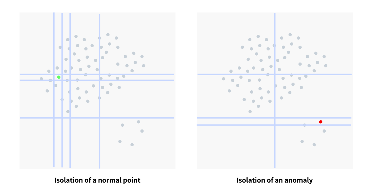
The diagram above shows the number of splits required to isolate a normal point and an anomaly. Splits, represented through blue lines, happens at random on a random attribute and in the process building a decision tree. The number of splits determines the level at which the isolation happened and will be used to generate the anomaly score.

The process is repeated multiple times and we note the isolation level for each point/instance. Once the iterations are over, we generate an anomaly score for each point/instance, suggesting its likeliness to be an anomaly. The score is a function of the average level at which the point was isolated. The top m gathered on the basis of the score, are labeled as anomalies.

Construction of decision tree

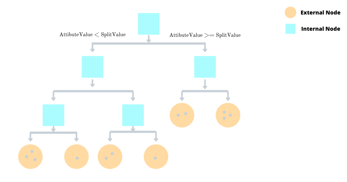
The decision tree is constructed by splitting the sub-sample points/instances over a split value of a randomly selected attribute such that the instances whose corresponding attribute value is smaller than the split value goes left and the others go right, and the process is continued recursively until the tree is fully constructed. The split value is selected at random between the minimum and maximum values of the selected attribute.

There are two types of node in the decision tree

Internal Node

Internal nodes are non-leaf and contain the split value, split attribute and pointers to two child sub-trees. An internal node is always a parent to two child sub-trees making the entire decision tree a proper binary tree.

External Node

External nodes are leaf nodes that could not be split further and reside at the bottom of the tree. Each external node will hold the size of the un-built subtree which is used to calculate the anomaly score.

Why sub-sampling helps

The Isolation Forest algorithm works well when the trees are created, not from the entire dataset, but from a sub-sampled data set. This is very different from almost all other techniques where they thrive on data and demands more of it for greater accuracy. Sub-sampling works wonder in this algorithm because normal instances can interfere with the isolation process by being a little closer to the anomalies.

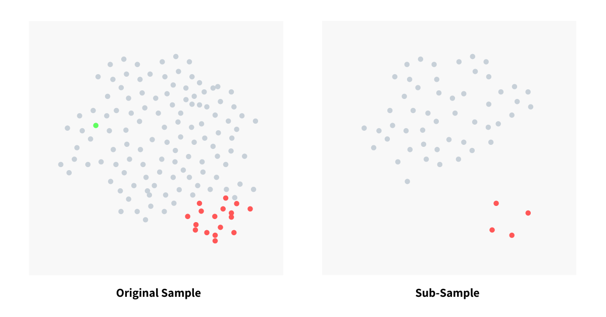
The image above shows how sub-sampling actually makes a clear separation between normal points and anomalies. In the original dataset, we see that normal points and very close to anomalies making detection tougher and inaccurate (with a lot of false negatives). Because of sub-sampling, we could see a clear separation of anomalies and normal instances. This makes the entire process of anomaly detection efficient and accurate.

Optimizing decision tree construction

Since anomalies are susceptible to isolation and have a tendency to reside closer to the root of the decision tree, we construct the decision tree till it reaches a certain height max_height and not split points further. This height is the height post which we are (almost) sure that there could not be any anomalies.

def construct_tree(X, current_height, max_height):
  """The function constructs a tree/sub-tree on points X.

  current_height: represents the height of the current tree to
    the root of the decision tree.
  max_height: the max height of the tree that should be constructed.

  The current_height and max_height only exists to make the algorithm efficient
  as we assume that no anomalies exist at depth >= max_height.
  """
  if current_height >= max_height:
    # here we are sure that no anomalies exist hence we
    # directly construct the external node.
    return new_external_node(X)

  # pick any attribute at random.
  attribute = get_random_attribute(X)

  # for set of inputs X, for the tree we get a random value
  # for the chosen attribute. preferably around the median.
  split_value = get_random_value(max_value, min_value)

  # split X instances based on `split_values` into Xl and Xr
  Xl = filter(X, lambda x: X[attribute] < split_value)
  Xr = filter(X, lambda x: X[attribute] >= split_value)

  # build an internal node with its left subtree created from Xl
  # and right subtree created from Xr, recursively.
  return new_internal_node(
    left=construct_tree(Xl, current_height + 1, max_height),
    right=construct_tree(Xr, current_height + 1, max_height),
    split_attribute=attribute,
    split_value=split_value,
  )

Constructing the forest

The process of tree construction is repeated multiple times and each time we pick a random sub-sample and construct the tree. There are no strict rules to determine the number of iterations, but in general, we could say the more the merrier. The sub-sampling count is also a parameter and could change depending on the data set.

The pseudocode for forest construction is as follows

def construct_forest(X, trees_count, subsample_count):
  """The function constructs a forest from given inputs/data points X.
  """
  forest = []
  for i in range(0, trees_count):
    # max_height is in fact the average height of the tree that would be
    # constructed from given points. This acts as max_height for the
    # construction because we are only interested in data points that have
    # shorter-than-average path lengths, as those points are more likely
    # to be anomalies.
    max_height = math.ceil(math.log2(subsample_count))

    # create a sample with cardinality of `subsample_count` from X
    X_sample = get_sample(X, subsample_count)

    # construct the decision tree from the sample
    tree = construct_tree(X_sample, 0, max_height)

    # add the tree to the forest
    forest.append(tree)

  return forest

While constructing the tree we pass max_height as log2(nodes_count) as that is the average height of a proper binary tree that could be constructed from nodes_count number of nodes. Since anomalies reside closer to the root node it is highly unlikely that any anomaly will isolate after the tree has reached height max_height. This helps us save a lot of computation and tree construction making it computationally and memory efficient.

Scoring the anomalies

Every anomaly detection algorithm has to score its data points/instances and quantify the confidence the algorithm has on its potential anomalies. The generated anomaly score has to be bounded and comparable. In Isolation Forest, that fact that anomalies always stay closer to the root, becomes our guiding and defining insight that will help us build a scoring function. The anomaly score will a function of path length which is defined as

Path Length h(x) of a point x is the number of edges x traverses from the root node.

As the maximum possible height of the tree grows by order of n, the average height grows by log(n) - this makes normalizing of the scoring function a little tricky. To remedy this we use the insights from the structure of the decision tree. The decision tree has two types of nodes internal and external such that external has no child while internal is a parent to exactly two nodes - which means the decision tree is a proper binary tree and hence we conclude

The average path length h(x) for external node termination is the same as the average path length of unsuccessful search in BST.

In a BST, an unsuccessful search always terminates at a NULL pointer and if we treat external node of the decision tree as NULL of BST, then we could say that average path length of external node termination is same as average path length of unsuccessful search in BST (constructed only from internal nodes of the decision tree), and it is given by

where H(i) is the harmonic number and it can be estimated by ln(i) + 0.5772156649 (Euler–Mascheroni constant). c(n) is the average of path length h(x) given n, we use it to normalize h(x).

To understand the derivation in detail refer to the references at the end of this article.

The anomaly score of an instance x is defined as

where E(h(x)) is the average path length (average of h(x)) from a collection of isolation trees. From the scoring function defined above, we could deduce that if

• the score is very close to 1, then they are definitely anomalies
• the score is much smaller than 0.5, then they are quite safe to be regarded as normal instances, and
• all the instances return around 0.5, then the entire sample does not really have any distinct anomaly

Evaluating anomalies

In the evaluation stage, an anomaly score is derived from the expected path length E(h(x)) for each test instance. Using get_path_length function (pseudocode below), a single path length h(x) is calculated by traversing through the decision tree.

If iteration terminates at an external node where size > 1 then the return value is e (number of edges traversed till current node) plus an adjustment c(size), estimated from the formula above. This adjustment is for the unbuilt decision tree (for efficiency) beyond the max height. When h(x) is obtained for each node of each tree, an anomaly score is produced by computing s(x, sample_size). Sorting instances by the score s in descending order and getting top m will yield us m anomalies.

def get_path_length(x, T, e):
  """The function returns the path length h(x) of an instance
  x in tree `T`.

  here e is the number of edges traversed from the root till the current
  subtree T.
  """
  if is_external_node(T):
    # when T is the root of an external node subtree
    # we estimate path length and return.

    # here c is the function which estimates the average path length
    # for external node termination.
    return e + c(len(T))

  # T is the root of an internal node then we
  if x[T.split_attribute] < T[split_value]:
    # instance x may lie in left subtree
    return get_path_length(x, T.left, e + 1)
  else:
    # instance x may lie in right subtree
    return get_path_length(x, T.right, e + 1)

References for BST unsuccessful search estimation

• IIT KGP, Algorithms, Lecture Notes - Page 7
• What is real big-O of search in BST?
• CMU CMSC 420: Lecture 5 - Slide 13
• CISE UFL: Data Structures, Algorithms, & Applications - 1st Proof

Conclusion

The isolation forest algorithm thrives on sub-sampled data and does not need to build the tree from the entire data set; it works well with sub-sampled data. While constructing the tree, we need not build tree taller than max_height (very cheap to compute), making it low on memory footprint. Since the algorithm does not depend on computationally expensive operations like distance or density calculation, it executes really fast. The training stage has a linear time complexity with a low constant and hence could be used in a real-time online system.

I hope this article helped you to understand Isolation Forest, an unsupervised anomaly detection algorithm. I stumbled upon this through an engineering blog of Grofers. This algorithm was very interesting to me because of its novel approach and hence I dived deep into it. FYI: In 2018, Isolation Forest was extended by Sahand Hariri, Matias Carrasco Kind, Robert J. Brunner. I have not read the Extended Isolation Forest algorithm but have definitely added it to my reading list. I recommend that if you liked this algorithm you should definitely give the extended version a skim.

This article was originally published on my blog - Isolation Forest algorithm for anomaly detection .

_If you liked what you read, subscribe to my newsletter and get the post delivered directly to your inbox and give me a shout-out @arpit_bhayani._