This article was originally written by MJ Bahmani and posted on the Neptune blog.

I've been using lightGBM for a while now. It's been my go-to algorithm for most tabular data problems. The list of awesome features is long and I suggest that you take a look if you haven't already. But I was always interested in understanding which parameters have the biggest impact on performance and how I should tune lightGBM parameters to get the most out of it. I figured I should do some research, understand more about lightGBM parameters… and share my journey. Specifically I:

Took a deep-dive into LightGBM's documentation
Went through Laurae articles Lauraepp: xgboost / LightGBM parameters
Looked into the LightGBM GitHub Repository
Ran some experiments myself

As I was doing that I gained a lot more knowledge about lightGBM parameters. My hope is that after reading this article you will be able to answer the following questions:

Which Gradient Boosting methods are implemented in LightGBM and what are its differences?
Which parameters are important in general?
Which regularization parameters need to be tuned?
How to tune lightGBM parameters in python?

Gradient Boosting methods

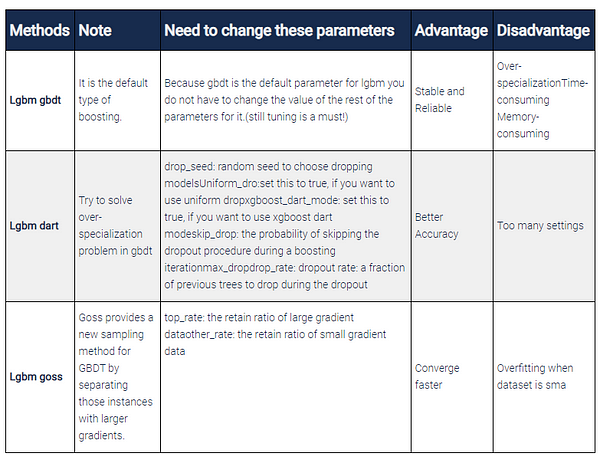
With LightGBM you can run different types of Gradient Boosting methods. You have: GBDT, DART, and GOSS which can be specified with the "boosting" parameter. In the next sections, I will explain and compare these methods with each other.

lgbm gbdt (gradient boosted decision trees)

This method is the traditional Gradient Boosting Decision Tree that was first suggested in this article and is the algorithm behind some great libraries like XGBoost and pGBRT. These days gbdt is widely used because of its accuracy, efficiency, and stability. You probably know that gbdt is an ensemble model of decision trees but what does it mean exactly? Let me give you a gist. It is based on three important principles:

Weak learners (decision trees)
Gradient Optimization
Boosting Technique

So in the gbdt method we have a lot of decision trees(weak learners). Those trees are built sequentially:

first tree learns how to fit to the target variable
second tree learns how to fit to the residual (difference) between the predictions of the first tree and the ground truth
The third tree learns how to fit the residuals of the second tree and so on.

All those trees are trained by propagating the gradients of errors throughout the system. The main drawback of gbdt is that finding the best split points in each tree node is time-consuming and memory-consuming operation other boosting methods try to tackle that problem.

dart gradient boosting

In this outstanding paper, you can learn all the things about DART gradient boosting which is a method that uses dropout, standard in Neural Networks, to improve model regularization and deal with some other less-obvious problems. Namely, gbdt suffers from over-specialization, which means trees added at later iterations tend to impact the prediction of only a few instances and make a negligible contribution towards the remaining instances. Adding dropout makes it more difficult for the trees at later iterations to specialize on those few samples and hence improves the performance.

lgbm goss (Gradient-based One-Side Sampling)

In fact, the most important reason for naming this method lightgbm is using the Goss method based on this paper. Goss is the newer and lighter gbdt implementation (hence "light" gbm). The standard gbdt is reliable but it is not fast enough on large datasets. Hence, goss suggests a sampling method based on the gradient to avoid searching for the whole search space. We know that for each data instance when the gradient is small that means no worries data is well-trained and when the gradient is large that should be retrained again. So we have two sides here, data instances with large and small gradients. Thus, goss keeps all data with a large gradient and does a random sampling (that's why it is called One-Side Sampling) on data with a small gradient. This makes the search space smaller and goss can converge faster. Finally, for gaining more insight about goss, you can check this blog post. Let's put those differences in a table:

Note: If you set boosting as RF then the lightgbm algorithm behaves as random forest and not boosted trees! According to the documentation, to use RF you must use bagging_fraction and feature_fraction smaller than 1.

Regularization

In this section, I will cover some important regularization parameters of lightgbm. Obviously, those are the parameters that you need to tune to fight overfitting.

You should be aware that for small datasets (<10000 records) lightGBM may not be the best choice. Tuning lightgbm parameters may not help you there.

In addition, lightgbm uses leaf-wise tree growth algorithm whileXGBoost uses depth-wise tree growth. Leaf-wise method allows the trees to converge faster but the chance of over-fitting increases.

Maybe this talk from one of the PyData conferences gives you more insights about Xgboost and Lightgbm. Worth to watch!

https://youtu.be/5CWwwtEM2TA

Note: If someone asks you what is the main difference between LightGBM and XGBoost? You can easily say, their difference is in how they are implemented.

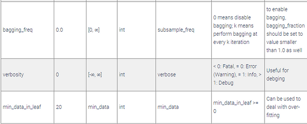
According to lightGBM documentation, when facing overfitting you may want to do the following parameter tuning:

Use small max_bin
Use small num_leaves
Use min_data_in_leaf and min_sum_hessian_in_leaf
Use bagging by set bagging_fraction and bagging_freq
Use feature sub-sampling by set feature_fraction
Use bigger training data
Try lambda_l1, lambda_l2 and min_gain_to_split for regularization
Try max_depth to avoid growing deep tree

In the following sections, I will explain each of those parameters in a bit more detail.

lambda_l1

Lambda_l1 (and lambda_l2) control to l1/l2 and along with min_gain_to_split are used to combat over-fitting. I highly recommend you to use parameter tuning (explored in the later section) to figure out the best values for those parameters.

num_leaves

Surely num_leaves is one of the most important parameters that controls the complexity of the model. With it, you set the maximum number of leaves each weak learner has. Large num_leaves increases accuracy on the training set and also the chance of getting hurt by overfitting. According to the documentation, one simple way is that num_leaves = 2^(max_depth) however, considering that in lightgbm a leaf-wise tree is deeper than a level-wise tree you need to be careful about overfitting! As a result, It is necessary to tune num_leaves with the max_depth together.

Photo on lightgbm documentation

subsample

With subsample (or bagging_fraction) you can specify the percentage of rows used per tree building iteration. That means some rows will be randomly selected for fitting each learner (tree). This improved generalization but also speed of training.

I suggest using smaller subsample values for the baseline models and later increase this value when you are done with other experiments (different feature selections, different tree architecture).

feature_fraction

Feature fraction or sub_feature deals with column sampling, LightGBM will randomly select a subset of features on each iteration (tree). For example, if you set it to 0.6, LightGBM will select 60% of features before training each tree. There are two usage for this feature:

Can be used to speed up training
Can be used to deal with overfitting

max_depth

This parameter control max depth of each trained tree and will have impact on:

The best value for the num_leaves parameter
Model Performance
Training Time

Pay attention If you use a large value of max_depth, your model will likely be over fit to the train set.

max_bin

Binning is a technique for representing data in a discrete view (histogram). Lightgbm uses a histogram based algorithm to find the optimal split point while creating a weak learner. Therefore, each continuous numeric feature (e.g. number of views for a video) should be split into discrete bins.

The photo on LightGBM and XGBoost Explained

Also, in this GitHub repo, you can find some comprehensive experiments which completely explains the effect of changing max_bin on CPU and GPU.

Clock time after 500 iterations - GitHub repo

If you define max_bin 255 that means we can have a maximum of 255 unique values per feature. Then Small max_bin causes faster speed and large value improves accuracy.

Training parameters

Training time! When you want to train your model with lightgbm, Some typical issues that may come up when you train lightgbm models are:

Training is a time-consuming process
Dealing with Computational Complexity (CPU/GPU RAM constraints)
Dealing with categorical features
Having an unbalanced dataset
The need for custom metrics
Adjustments that need to be made for Classification or Regression problems

In this section, we will try to explain those points in detail.

num_iterations

Num_iterations specifies the number of boosting iterations (trees to build). The more trees you build the more accurate your model can be at the cost of:

Longer training time
Higher chance of overfitting

Start with a lower number of trees to build a baseline and increase it later when you want to squeeze the last % out of your model. It is recommended to use smaller learning_rate with larger num_iterations. Also, you should use early_stopping_rounds if you go for higher num_iterations to stop your training when it is not learning anything useful.

early_stopping_rounds

This parameter will stop training if the validation metric is not improving after the last early stopping round. That should be defined in pair with a number of iterations. If you set it too large you increase the change of overfitting (but your model can be better).

The rule of thumb is to have it at 10% of your num_iterations.

lightgbm categorical_feature

One of the advantages of using lightgbm is that it can handle categorical features very well. Yes, this algorithm is very powerful but you have to be careful about how to use its parameters. lightgbm uses a special integer-encoded method (proposed by Fisher) for handling categorical features

Experiments show that this method brings better performance than, often used, one-hot encoding.

The default value for it is "auto" that means: let lightgbm decide which means lightgbm will infer which features are categorical.

It doesn't always work well (some experiment show why here and here) and I highly recommend you set categorical feature manually simply with this code

cat_col = dataset_name.select_dtypes('object').columns.tolist()

But what happens behind the scenes and how lightgbm deals with the categorical features?

According to the documentation of lightgbm, we know that tree learners cannot work well with one hot encoding method because they grow deeply through the tree. In the proposed alternative method, tree learners are optimally constructed. For example for one feature with k different categories, there are 2^(k-1) - 1 possible partition and with fisher method that can improve to k * log(k) by finding the best-split way on the sorted histogram of values in the categorical feature.

lightgbm is_unbalance vs scale_pos_weight

One of the problems you may face in the binary classification problems is how to deal with the unbalanced datasets. Obviously, you need to balance positive/negative samples but how exactly can you do that in lightgbm?

There are two parameters in lightgbm that allow you to deal with this issue is_unbalance and scale_pos_weight, but what is the difference between them and How to use them?

When you set Is_unbalace: True, the algorithm will try to Automatically balance the weight of the dominated label (with the pos/neg fraction in train set)
If you want change scale_pos_weight (it is by default 1 which mean assume both positive and negative label are equal) in case of unbalance dataset you can use following formula(based on this issue on lightgbm repository) to set it correctly

sample_pos_weight = number of negative samples / number of positive samples

lgbm feval

Sometimes you want to define a custom evaluation function to measure the performance of your model you need to create a "feval" function. Feval function should accept two parameters:

preds
train_data

and return

eval_name
eval_result
is_higher_better

Let's create a custom metrics function step by step.

Define a separate python function

def feval_func(preds, train_data):
   # Define a formula that evaluates the results
    return ('feval_func_name', eval_result, False)

Use this function as a parameter:

print('Start training...')
lgb_train = lgb.train(..., 
                      metric=None, 
                      feval=feval_func)

Note: to use feval function instead of metric, you should set metric parameter "None".

classification params vs regression params

Most of the things I mentioned before are true both for classification and regression but there are things that need to be adjusted. Specifically you should:

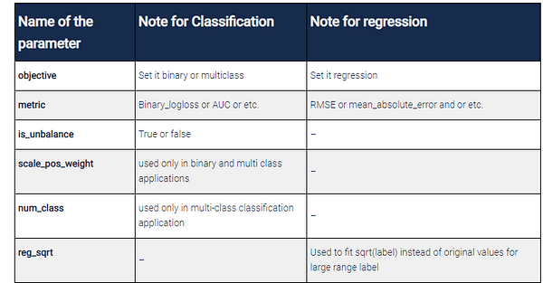
The most important lightgbm parameters

We have reviewed and learned a bit about lightgbm parameters in the previous sections but no boosted trees article would be complete without mentioning the incredible benchmarks from Laurae 🙂

You can learn about best default parameters for many problems both for lightGBM and XGBoost.

You can check it out here but some most important takeaways are:

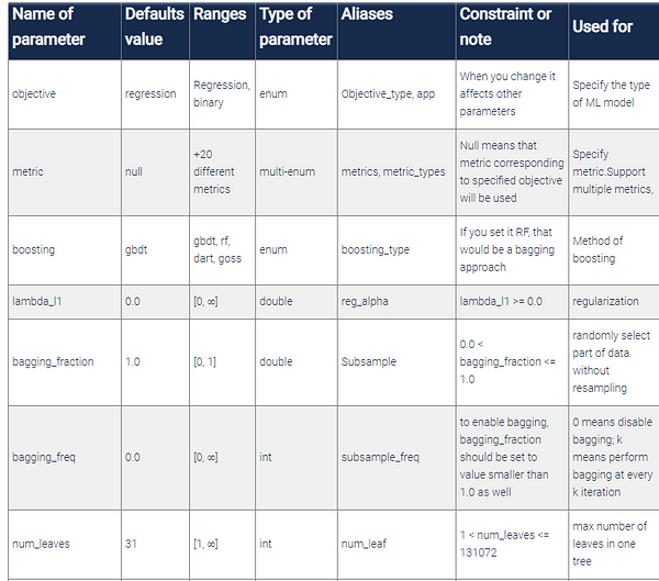
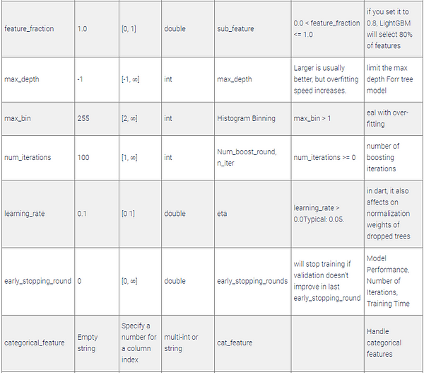
Note: You should never take any parameter value for granted and adjust it based on your problem. That said, those parameters are a great starting point for your hyperparameter tuning algorithms.

Lightgbm parameter tuning example in Python (lightgbm tuning)

Finally, after the explanation of all important parameters, it is time to perform some experiments!

I will use one of the popular Kaggle competitions: Santander Customer Transaction Prediction.

I will use this article which explains how to run hyperparameter tuning in Python on any script.

Worth a read!

Before we start, one important question! What parameters should we tune?

Pay attention to the problem you want to solve, for instance Santander dataset is highly imbalanced, and should consider that in your tuning! Laurae2, one of the contributors to lightgbm, explained this well here.
Some parameters are interdependent and must be adjusted together or tuned one by one. For instance, min_data_in_leaf depends on the number of training samples and num_leaves.

Note: It's a good idea to create two dictionaries for hyperparameters, one contains parameters and values that you don't want to tune, the other contains parameter and value ranges that you do want to tune.

SEARCH_PARAMS = {'learning_rate': 0.4,
                 'max_depth': 15,
                 'num_leaves': 20,
                 'feature_fraction': 0.8,
                 'subsample': 0.2}

FIXED_PARAMS={'objective': 'binary',
              'metric': 'auc',
              'is_unbalance':True,
              'boosting':'gbdt',
              'num_boost_round':300,
              'early_stopping_rounds':30}

By doing that you keep your baseline values separated from the search space!

Now, here's what we'll do.

First, we generate the code in the Notebook. It is public and you can download it.
Second, we track the result of each experiment on Neptune.ai.

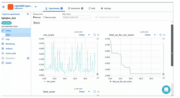
analysis of results

If you have checked the previous section, you've noticed that I've done more than 14 different experiments on the dataset. Here I explain how to tune the value of the hyperparameters step by step. Create a baseline training code:

from sklearn.metrics import roc_auc_score, roc_curve
from sklearn.model_selection import train_test_split
import neptunecontrib.monitoring.skopt as sk_utils
import lightgbm as lgb
import pandas as pd
import neptune
import skopt
import sys
import os

SEARCH_PARAMS = {'learning_rate': 0.4,
                'max_depth': 15,
                'num_leaves': 32,
                'feature_fraction': 0.8,
                'subsample': 0.2}

FIXED_PARAMS={'objective': 'binary',
             'metric': 'auc',
             'is_unbalance':True,
             'bagging_freq':5,
             'boosting':'dart',
             'num_boost_round':300,
             'early_stopping_rounds':30}

def train_evaluate(search_params):
   # you can download the dataset from this link(https://www.kaggle.com/c/santander-customer-transaction-prediction/data)
   # import Dataset to play with it
   data= pd.read_csv("sample_train.csv")
   X = data.drop(['ID_code', 'target'], axis=1)
   y = data['target']
   X_train, X_valid, y_train, y_valid = train_test_split(X, y, test_size=0.2, random_state=1234)
   train_data = lgb.Dataset(X_train, label=y_train)
   valid_data = lgb.Dataset(X_valid, label=y_valid, reference=train_data)

   params = {'metric':FIXED_PARAMS['metric'],
             'objective':FIXED_PARAMS['objective'],
             **search_params}

   model = lgb.train(params, train_data,                     
                     valid_sets=[valid_data],
                     num_boost_round=FIXED_PARAMS['num_boost_round'],
                     early_stopping_rounds=FIXED_PARAMS['early_stopping_rounds'],
                     valid_names=['valid'])
   score = model.best_score['valid']['auc']
   return score

Use the hyperparameter optimization library of your choice (for example scikit-optimize)

neptune.init('mjbahmani/LightGBM-hyperparameters')
neptune.create_experiment('lgb-tuning_final', upload_source_files=['*.*'],
                              tags=['lgb-tuning', 'dart'],params=SEARCH_PARAMS)

SPACE = [
   skopt.space.Real(0.01, 0.5, name='learning_rate', prior='log-uniform'),
   skopt.space.Integer(1, 30, name='max_depth'),
   skopt.space.Integer(10, 200, name='num_leaves'),
   skopt.space.Real(0.1, 1.0, name='feature_fraction', prior='uniform'),
   skopt.space.Real(0.1, 1.0, name='subsample', prior='uniform')
]
@skopt.utils.use_named_args(SPACE)
def objective(**params):
   return -1.0 * train_evaluate(params)

monitor = sk_utils.NeptuneMonitor()
results = skopt.forest_minimize(objective, SPACE, 
                                n_calls=100, n_random_starts=10, 
                                callback=[monitor])
sk_utils.log_results(results)

neptune.stop()

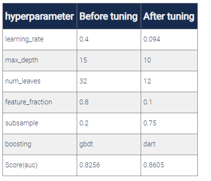
Try different types of configuration and track your results in Neptune

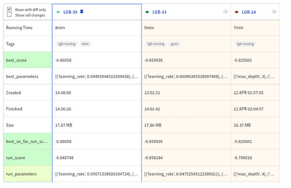
Finally, in the following table, you can see what changes have taken place in the parameters.

Final Thoughts:

Long story short, you learned:

what the main lightgbm parameters,
how to create custom metrics with the feval function
what are the good default values of major parameters
saw and example of how to tune lightgbm parameters to improve model performance

And some other things 🙂 For more detailed information, please refer to the resources.

Resources:

This article was originally written by MJ Bahmani and posted on the Neptune blog. You can find there more in-depth articles for machine learning practitioners.

Understanding LightGBM Parameters (and How to Tune Them)