Neural Network by Chesta Dhingra

Neural Network is the software implementation of neuronal structure of our brains. This enables a computer to learn from the observational data which we called as supervised learning. It’s not only used in supervised learning but also in unsupervised learning. The supervised learning takes place by adjusting the weights of the connections whereas unsupervised learning is an attempt to help the model in understanding the structure of the input data on its own.

In supervised learning we already have the labels on the data which differentiates between the independent variables (which helps in predicting the value of dependent variable) and the dependent variable denoted as ”Y”. It’s a learning algorithm which iteratively makes predictions on the training data and stops when it achieves an acceptable level of performance.

In unsupervised learning we only have the input data and no corresponding output variable is present. In this type of learning the data has to make the groupings by iteratively running the algorithms and do the clustering based on the similarities among the variables.

This Artificial Neural Network also knows as ANN this comprised of large number of simple elements called neurons and composed of four principal objects:- • Layers: - All learning of the model occurs in the layers. The three most important layers are ◦ 1) Input Layer ◦ 2) Hidden layer ◦ 3) Output Layer

• Features and Labels: - input data which is provided to the network is called as “features” and the output from the network is called as “labels”
• Loss function: - It’s a metric used to estimate the performance of learning phase.
• Optimizer: - it improves learning by updating the knowledge in the network.

A brief summary of overall process before diving deep into the world of Artificial Neural Network is that, Firstly the input data is pushed into the ensemble layers further the performance is evaluated by the loss function which provides an idea to the network which path it needs to take before making its solid assumptions or mastering its knowledge. Lastly it improves its knowledge by using the optimizer which helps the model in minimizing the errors.

Layers consist of nodes which we also called as “perceptron”. First layer is consists of a group of input nodes altogether known as input layer which contains the actual data from the outside world. No computation has been performed on these input layers only the flow of information or passing of information would take place. Then have the “Hidden Nodes” collectively known as “hidden layer” in which computation will performed and then transfer the information from input node to the output nodes. It doesn’t have any direct connection with the outside world.

A neural network can have single input layer and output layer with zero hidden layers or it might have one or more than one hidden layers in the network. Lastly have the “Output Nodes” which are collectively called as “Output Layer” and are responsible for computations and transferring the information from the network to the outside world.

Layers are the one where all learning takes place. Infinite amounts of weights are there which we termed as “weights”. These nodes are densely connected with each other and each node takes multiple weighted inputs, applies this activation function to the summation of these inputs and then generates the output. These weights are the real numbers which are multiplied by the inputs and summed up in the node. The equation would be like: x1w1+x2w2+x3w3+b

Where w1 is the weight or the variable which changed during the learning process along with the input and on the basis of that determines the output. The b is the +1bias element which helps in enhancing the flexibility of the node. The weights change the slope of activation function.

Activation function defines the output given set of inputs. We need the activation function so network will able to learn the non linear pattern. Most commonly used activation function is “Relu”known as rectified linear unit which gives zero for all negative values. R (z) = max (0, z)

Some of the other activation functions are:- • Sigmoid function: - this function exists between 0 and 1 especially for models where we have to define the probability. It produces the clear predictions for x but it brings the value for y very close to 0 and 1.

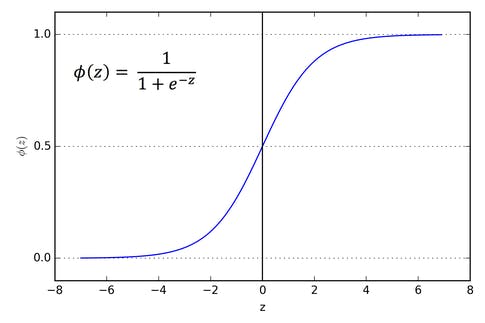
Sigmoid Function

• Tanh – this is better than the sigmoid as it range from -1 to 1 on the y axis. Here negative is mapped strongly negative and zero inputs will mapped near zero in the tanh graph. This produces the zero concentrated graphs.

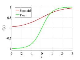
Tanh Function

• Leaky Relu – It increased the range of ReLU function as in the ReLU the f(y) = 0 when have the negative value but in Leky ReLU f(y) = ay, here a is 0.01 and when it is not 0.01 then it is known as “Randomized ReLU”. Therefore, range of Leaky ReLU is negative infinity to positive infinity.

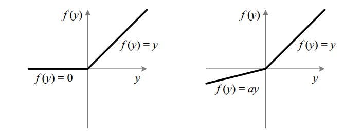1) ReLU Function 2) Leky ReLU The bias is not the true node with the activation function thus have no inputs. The process of calculating the output with these values is called the “feed forward process”. As per the difference that I am able to understand between introducing weights and bias is that weight is applied on the layers whereas the bias is applied in each node and can change when the node activates. Therefore by adding the bias term, we can make node simulate the generic if function, i.e. if(x>z) 1 else 0. By summing up all the values we get the equation

h (2)1=f(w(1)11x1+w(1)12x2+w(1)13x3+b(1)1) h (2)2=f(w(1)21x1+w(1)22x2+w(1)23x3+b(1)2) h (2)3=f(w(1)31x1+w(1)32x2+w(1)33x3+b(1)3) hW,b(x)=h(3)1=f(w(2)11h(2)1+w(2)12h(2)2+w(2)13h(2)3+b(2)1)

where f is the activation function w is the weight and b is the bias. The h (2)1 is the output of the first node in the second layer and the inputs are
w(1)11x1+w(1)12x2+w(1)13x3+b(1)1

The same thing goes for the other two nodes and lastly the final line is the output of only node in the third and final layer, which is the ultimate output of the neural network.

Loss function is a method of evaluating how well your algorithms model your data set. If predictions are totally off then you will get a higher number of output. If the model is pretty good it will let you know by giving the output lower in number. It’s not just the static representation of how the model is performing they let us know that how the algorithm fits the data in the first place. Different types of loss functions are: -

• Mean Squared Error – it’s the squared distance between target variable and predicted values. It is mostly used in regression loss. To calculate MSE, take out the difference between the predictions and the actual values, square it, and average it out across the whole dataset.

• Likelihood Loss – it is used in classification problems. The function takes the predicted probability for each input example and multiplies them.

• Log Loss (Cross Entropy Loss) – each predicted probability is compared to actual class output value (0 or 1) and score is calculated that penalizes the probability based on the distance from expected value. Probability is logarithmic differing a small score for small value (0.1 or 0.2) and enormous score for large value (0.9 or 1.0). The loss is minimized when smaller values represent the better score. Model which is able to predict better probabilities has a cross entropy or log loss of 0.0. It is also known as “Logarithmic loss” or “Logistic Loss”

Lastly, the optimizer which helps in improving the model or network. Generally the “Gradient Descent “optimization algorithm used to minimize the function by iteratively moving in the direction of steepest descent as defined by negative of the gradient. The main idea is to reduce error between the input and the desired output. In this the error is depend on the weight w in the network so the motive is to get the minimum possible error by starting out random value of “w”so that it will reach at the optimum value.

The gradient also helps in finding the direction if it is positive with respect to increase in w than increase in that step leads to increase in error as well, if its negative in respect to increase in value of w than it will lead to decrease in error. The magnitude of the gradient or the steepness will help us to give information that how fast is the error curve or function is changing. The higher the magnitude the faster the error is changing at that point with respect to w.